Tutorial

This page provides a tutorial for multi-tissue TWAS fine-mapping using mFABIO. Before runing the example code, make sure that the mFABIO software is installed successfully. For instructions on installation, please see the Installation section.

mFABIO #

The example data for mFABIO tutorial can be accessed following this page. Here are the details about the input data formats and how to run mFABIO.

1. Format of input for mFABIO #

• Predicted GReX: We require the predicted GReX of the TWAS cohort built up using standard softwares like SuSiE. The input GReX is expected to be a R matrix, which has column names in the format of [Tissue Name]-[Gene Name/ID]. No requirement on the row names of this R matrix. An example data matrix can be found here:

  library(mFABIO)
  data(example_data)
  > dim(example_data$G)
  [1] 2000  300
  > example_data$G[1:5,1:5]
     Tissue1-Gene001 Tissue2-Gene001 Tissue3-Gene001 Tissue4-Gene001 Tissue5-Gene001
  [1,]      -0.7550567     -1.42914073     -0.88960517     -0.11741247      -0.4213615
  [2,]       0.8011494      0.32952949     -0.14682934     -0.07053631       0.1506835
  [3,]       0.5685453      0.33475624      0.01785558      0.17683326       0.1383405
  [4,]       0.6705940      0.99009064     -0.47588513      0.33221315       0.5847007
  [5,]      -0.4316600     -0.07432518      0.62807354     -1.01307066      -0.5182504
  

• Binary phenotypes: We also require the observed binary phenotypes of the TWAS cohort. The input phenotypes are expected as a R vector, with 1 coding for case and 0 for control. The order of the individuals here should be consistent with the order of rows in the predicted GReX matrix. An example can be found here:

  > dim(example_data$y)
  [1] 2000    1
  > head(example_data$y)
     [,1]
  [1,]    1
  [2,]    1
  [3,]    1
  [4,]    0
  [5,]    1
  [6,]    1
  

• Genotypes of cis-SNPs (optional): You may include the genotypes of all the cis-SNPs used in predicting GReX to account for pleiotropic effects. The input genotypes are expected as a R matrix with no requirements on the row or column names, but the row order of the individuals here should be consistent with that in the predicted GReX matrix as well as the phenotype vector. An example can be found here:

  > dim(example_data$X)
  [1] 2000 1000
  > example_data$X[1:5,1:5]
          [,1]       [,2]       [,3]        [,4]        [,5]
  [1,] -1.0357630 -0.0993181 -0.8196765 -1.04250565 -0.56026171
  [2,]  1.5967262  1.3356525 -0.3146939  0.81951812  0.87080511
  [3,]  0.6504174 -1.2835909 -0.5329149  0.25042639 -1.81556533
  [4,] -1.1285718 -0.4096962 -1.4196629  0.03090357 -0.07253444
  [5,]  0.3552911 -1.0795471  0.6296525 -0.62696991  0.63727596
  

2. Running mFABIO #

The multi-tissue TWAS fine-mapping can be performed using the following scripts with our example data:

res <- run_mfabio(G = example_data$G, y = example_data$y, X = example_data$X)

3. mFABIO output #

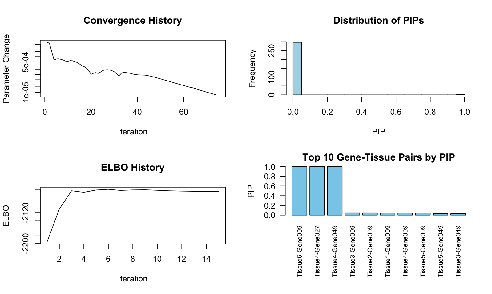
mFABIO will output a summary R list object. A diagnostic glance on the results can be extracted like this:

> res$plot_diagnostics()
# The true signals in our simulated example data are: Gene009 in Tissue6,
# Gene027 in Tissue4, and Gene049 in Tissue4.

The gene level PIPs can be extracted like this:

> sort(res$pip_gene, decreasing = T)[1:10]
   Gene009    Gene049    Gene027    Gene045    Gene030    Gene050    Gene031    Gene042    Gene005    Gene014 
0.09383752 0.03743529 0.03721592 0.01785030 0.01784515 0.01784478 0.01779710 0.01777913 0.01777440 0.01777248

The gene-tissue pair level PIPs can be extracted like this:

> sort(res$pip_pair, decreasing = T)[1:10]
Tissue6-Gene009 Tissue4-Gene027 Tissue4-Gene049 Tissue3-Gene009 Tissue2-Gene009 Tissue1-Gene009 Tissue4-Gene009 
     1.00000000      0.99999938      0.99995888      0.04793659      0.04769466      0.04675122      0.04575907 
Tissue5-Gene009 Tissue5-Gene049 Tissue3-Gene049 
     0.04569619      0.02861870      0.02824001